emobpy
emobpy is a Python tool that can create battery electric vehicle time series. Four different time series can be created: vehicle mobility time series, driving electricity consumption time series, grid availability time series and grid electricity demand time series. The vehicles mobility time series are created based on mobility statistics. For driving electricity consumption time series, the properties of vehicles can be selected from a database with several actual battery electric vehicles models. emobpy is developed by the research group Transformation of the Energy Economy at DIW Berlin (German Institute of Economic Research).
Note
Cite this article: Gaete-Morales, C., Kramer, H., Schill, WP. et al. An open tool for creating battery-electric vehicle time series from empirical data, emobpy. Sci Data 8, 152 (2021). https://doi.org/10.1038/s41597-021-00932-9
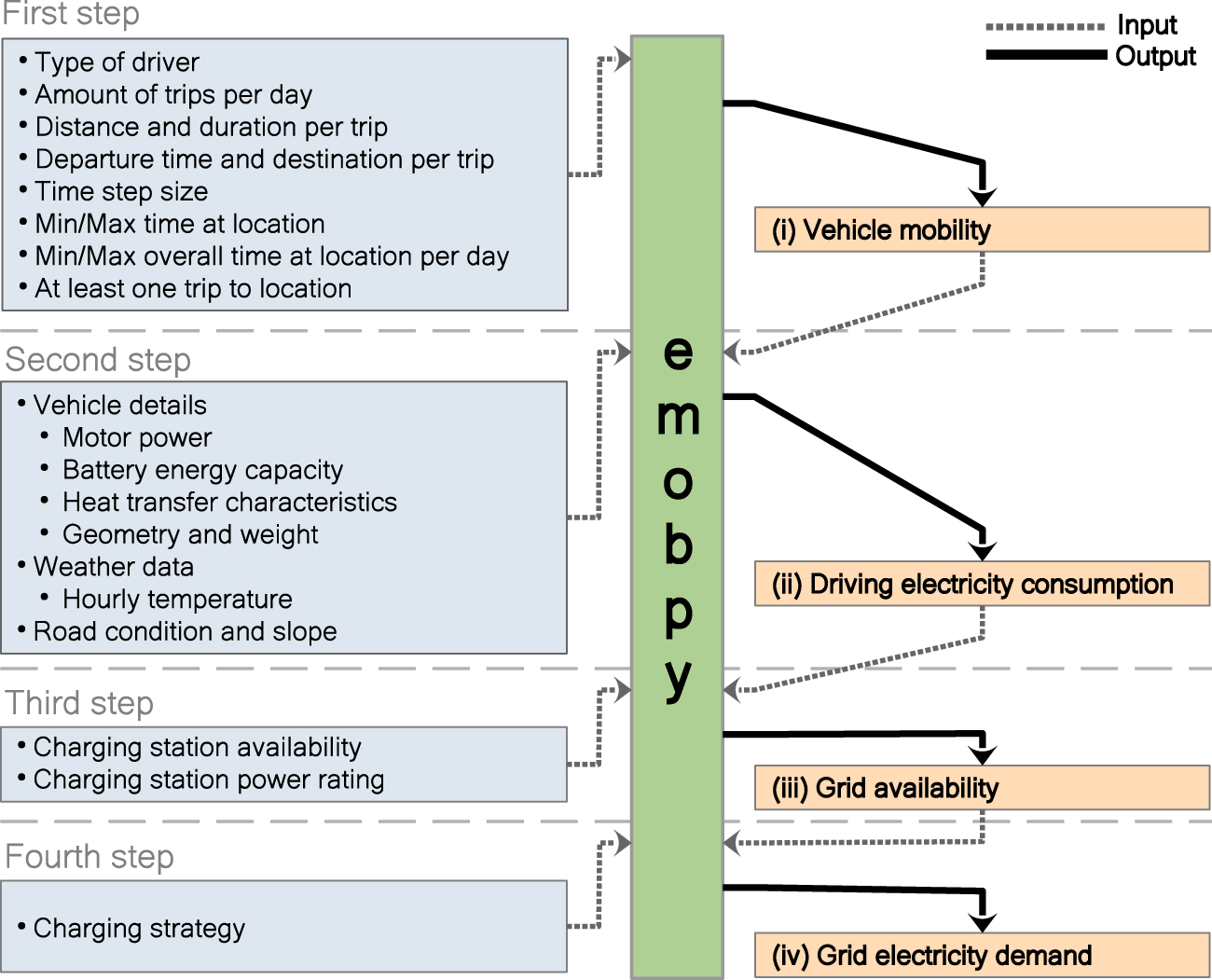
Vehicle mobility time series
The vehicle mobility time series contains the location of a vehicle at each point in time. The locations vary according to the mobility of drivers. Possible locations are at home, workplace, shopping, errands, escort, leisure, or driving. When “Driving”, the distance travelled is also provided in the time series. The time resolution can be established initially (our examples contains 15 minutes time steps). The daily number of trips, the departure time, the trip purpose, distance travelled, and duration of the trips are determined based on statistics of mobility surveys. Other considerations can also be set up. For instance, the number of working hours per day, the first and last destination of the day, can be established as “at home”. The “driving” will always be placed in between two different locations.
Driving electricity consumption time series
The previous time series is used as input to the creation of driving electricity consumption time series. The energy required for every trip is calculated based on the ambient temperature and traction effort for the vehicle’s movement. To simulate the travel conditions, driving cycles are taken into account. The tool counts with battery electric vehicle models that are currently in the market. A vehicle’s model has to be selected to include the model’s parameters and characteristics.
Grid availability time series
Grid availability time series consists of taking a driving electricity consumption time series and based on the locations. The model assigns charging stations. Different charging stations can be available for a vehicle, and they are chosen based on a probability distribution that adds up 100% for each location. The charging stations defined in this tool are “home”, “public”, “maker”, “workplace”, “fast” and “none”, although more user-defined charging stations can be established. The charging stations have an associated capacity per time interval, and “none” has zero capacity. Different scenarios of grid availability can be modelled.
Grid electricity demand time series
While a grid availability time series contains at each interval information of the charging stations available, such as the maximum power rating allocated to them, a grid electricity demand time series is the one that indicates the actual consumption of electricity from the grid to charge the battery of a vehicle according to its driving needs and grid availability. There are different options available to create a grid electricity demand time series. For example, “Immediate-Full capacity” is an option that informs the energy drawn from the grid at a maximum power rating of a respective charging station until the battery is fully charged or “Immediate-Balanced” option that creates a time series taking into account the duration of a vehicle is connected to a charging station and the energy required to get the battery fully charged, allowing to charge the battery at a lower capacity than the maximum capacity available.
Instructions
This tool has been tested in window 7, Ubuntu 18.04, Ubuntu 19.04 and Suse Linux. It is recommended to install the package in an dedicated Python environment with Python version 3.6+.
Installation:
Usage
You can use our project template. It is a folder that contains files with mobility probabilities, assumptions in a rules file and python scripts that show different python classes and functions to start generating the time series.
To get a copy of the template folder, we create a project folder. For instance, as shown below, our project name is my_evs.
Hint
When we create a project folder for the first time, emobpy also copies files to our system user folder. In windows is usually located in c:/users/your_win_user/AppData/Local/emobpy, while for Linux is /home/your_linux_user/.local/share/emobpy. The files hosted contain actual battery electric vehicle models, weather time series hourly across a year for different countries, and driving cycles divided on urban, rural, and highways.
Then by using the command line, we access to project folder my_evs:
We can run the python script that enables us to generate examples of time series.
read the instruction file in my_evs folder
Jupyter notebook offers a more interactive learning. You can open the Time-series_generation.ipynb
by running jupyter in your console.
In the example section of the documentation, the code is clearly explained. Go directly to the example here.
Remove library:
Authors
The developers are Carlos Gaete-Morales (lead) and Lukas Trippe.
Installation
To run emobpy, you should have a functioning installation of Python.
It is a good idea to install emobpy within a conda environment. The result can best be visualized in a jupyter notebook. However, it is also possible to run emobpy through other python interpreter.
The following instructions describes in detail how to install Python, how to create a conda
environment, and finally how to install emobpy and its dependencies.
This tool has been tested in window 7, Ubuntu 18.04, Ubuntu 19.04 and Suse Linux. Python version 3.6+.
Installation of Python with Conda
The easiest and most convenient way to install Python is to install Anaconda (or Miniconda). Download the latest version from their website and install it.
During the installation of Anaconda on Windows, you will be asked to specify several options. We recommend you to choose the following ones so that emobpy will run smoothly:
Install Anaconda to a custom directory (such as C:/Anaconda
or D:/Anaconda
) and do not install it in the default folder, because this might increase the log-in and log-out out time;
Do not use C:/Programs/
or C:/Program Files/
because this will require admin rights (recommended for permission restricted computers);
During the installation, select “advanced option” and check both boxes (despite not recommended by the application). This will add this Conda Python Installation to the path and enables it as default python.
Create a new Conda environment
An conda environment is an isolated Python space. Different environments can contain different Python packages of different versions. In order to have reproducible and stable “working space”, it is useful to create a new environment for emobpy.
Anaconda offers different ways to create a new environment:
1. Anaconda Navigator
Start the Anaconda Navigator and go on Environments and then create. Choose a name, tick the box next to Python and choose a Python version compatible with your GAMS installation (see box above).
2. Console
Open a console (Anaconda Prompt, CMD, PowerShell, Windows Terminal) and create a new conda environment with the name yourenvname and the exemplary Python version X.X (we recommend 3.6) with the following command:
$ conda create -n yourenvname python=X.X
Note
To verify the successful creation of your environment, type conda info --envs
in your console.
For further information on how to edit and delete conda environments, we refer to the conda documentation.
Installation of emobpy
Now, your are ready to install emobpy. Make sure you have activated the correct environment:
$ conda activate yourenvname
You can install emobpy easily from PyPI:
Installing emobpy from PyPI ensures that all necessary linked packages are downloaded and installed.
Note
You can uninstall emobpy, while having activated the yourenvname environment, simply by executing $ pip uninstall emobpy
in the console.
Creating a project folder
Before start creating time-series we have to create a new project folder. By creating a project we will copy all required files from a template folder. These files can be modified according to our research purpose.
In our example, we want to create a new project called my_evs and use the console to create the project folder. Open the console (or terminal) where you want to create the project folder (e.g. in Windows by right-clicking and shift and choosing Open Windows Terminal here), or navigate to the desired folder within the console.
Once you are in the desired folder and if emobpy was installed correctly, type the following command:
$ emobpy create -n my_evs
or:
$ emobpy create --name my_evs
Warning
The name of the project must not contain any blanks. This can lead to errors.
Further options
In addition, further settings can be made. For example, a seed can be set. This allows that the same calculations are always executed in the same way. This makes it easy to compare projects and simplifies further development. If no seed is given, it will be randomly generated.
Argument |
Shortcut |
Optional |
Description |
–name |
-n |
Required |
Name of the project folder. |
–template |
-t |
Optional |
Select a specific example project. |
–seed |
-s |
Optional |
Set a seed to make calculations reproducible. |
This will create a folder and file structure as follows.
├── my_evs
│ └── config_files
│ ├── DepartureDestinationTrip.csv
│ ├── DistanceDurationTrip.csv
│ ├── TripsPerDay.csv
│ ├── rules.yml
│ ├── Time-series_generation.ipynb
│ ├── Step1Mobility.py
│ ├── Step2DrivingConsumption.py
│ ├── Step3GridAvailability.py
│ ├── Step4GridDemand.py
│ ├── Visualize_and_Export.ipynb
To start creating the time series, follow the instructions on the next page.
Generate the time-series
After having created a project folder (previuos section), you are ready to run the model. This happens in four steps.
The information in this chapter can also be found in the Instruction.txt file that is created with the creation of a new project folder.
Base Case
If not already done, change to project folder:
Warning
It is recommended to perform the following steps only if a conda environment has been installed and activated. Instructions can be found in the Installation page.
Method 1: Jupyer Notebook
Once the browser opens up, select and open Time-series_generation.ipynb
.
Method 2: Python interprreter
Run the script in the following order:
$ python Step1Mobility.py
$ python Step2DrivingConsumption.py
$ python Step3GridAvailability.py
$ python Step4GridDemand.py
After finishing all the runs, open Visualize_and_Export.ipynb for visualization of results.
Warning
jupyter notebook must be installed, it can be installed conda install jupyter
.
Examples
This section contains examples developed to help understand the features and functionalities of emobpy. To facilitate the implementation and execution of the examples, the tool enables us to create projects from templates that contain such examples. We expect to provide more examples further forward.
To obtain the template of an example we have to run the command line interface as follows:
$ dieterpy create_project -n myproject -t eg1
In the above code snippet -n
is an argument to provide the name of our project myproject and -t
is the argument to provide the name of the template to obtain eg1.
Hint
If no template (-t) is provided dieterpy create_project -n myproject
, then the base case folder will be generated.
Base Case
This is the base case that will be created if no specific template is selected. It serves as a foundation for own modeling and to get an overview for the program.
To initialize the base case and create a project folder, no template needs to be specified:
$ emobpy create -n <give a name>
Hint
Before running this example, install and activate a dedicated environment (a conda environment is recommended).
The initialisation creates a folder and file structure as follows:
├── my_evs
│ └── config_files
│ ├── DepartureDestinationTrip.csv
│ ├── DistanceDurationTrip.csv
│ ├── TripsPerDay.csv
│ ├── rules.yml
│ ├── Time-series_generation.ipynb
│ ├── Step1Mobility.py
│ ├── Step2DrivingConsumption.py
│ ├── Step3GridAvailability.py
│ ├── Step4GridDemand.py
│ ├── Visualize_and_Export.ipynb
This base case consists of four .py files that run the modelling, a .ipynb to visualise the results and the config_files folder that contains mobility data.
File name |
Description |
config_files/
|
Mobility data files that can be changed in this folder. |
Step1Mobility.py
|
Uses emobpy.Mobility() to create individual mobility time series with
vehicle location and distance travelled. |
Step2DrivingConsumption.py
|
Uses emobpy.Consumption() to assign vehicles and to model their consumption. |
Step3GridAvailability.py
|
Uses emobpy.Availability() to create the grid availability time series. |
Step4GridDemand.py
|
Uses emobpy.Charging() to calculate the grid electricity demand time series. |
Visualize_and_export.ipynb
|
Jupyter Notebook File to view the results. See Visualization. |
Time-series_generation.ipynb
|
Jupyter Notebook File to create and visualize all four time series (Recomended). |
After initialisation, you have two options: Using jupyter notebook or the python interpreter directly.
Method 1: Using Jupyter notebook
It will open the notebook in your browser. The document contains all instructions.
Warning
Make sure you have installed jupyter in your activated environment. To install it type in the console conda install jupyter
The jupyter notebook file could look like this, for example:
Method 2: Python interpreter
Run the script in the following order:
$ cd <given name>
$ python Step1Mobility.py
$ python Step2DrivingConsumption.py
$ python Step3GridAvailability.py
$ python Step4GridDemand.py
The results are saved as pickle files. To read them, two methods can be implemented. Using the DataBase class as described in the Visualize_and_Export.ipynb or by opening the pickle file directly. More information can be found in the pickle documentation.
The pickle file can be opened as follows:
pickle_in = open("data.pickle","rb")
data = pickle.load(pickle_in)
The jupyter notebook file .ipynb file could look like this:
BEV models
This example shows the different cars that are included in the database. A Sankey diagram can be used to clearly identify the energy usage for each car.
To initialize the example1 and create a project folder, the template eg1 must be selected:
$ emobpy create -n <give a name> -t eg1
Warning
Before running this example, install and activate an emobpy dedicated environment (conda recommended).
The initialisation creates a folder and file structure as follows.
├── my_evs
│ └── config_files
│ ├── DepartureDestinationTrip_Worker.csv
│ ├── DistanceDurationTrip.csv
│ ├── rules.yml
│ ├── TripsPerDay.csv
│ ├── eg1.ipynb
Everything, running and visualization, happens in a single jupyter notebook file. In the default settings a single mobility profile is created and three consumption profiles for different car types. For each car a Sankey diagram is created to show the different energy usage of the cars.
The Jupyter notebook might look like this:
emobpy
emobpy package
emobpy.availability module
emobpy.consumption module